Why a One-Line Baseline Does Well on Time Series Anomaly Detection Benchmarks: A Follow-up to Wu and Keogh

A note on audience. This post is written for undergraduates who have finished their introductory machine learning courses and are looking at research areas to work in. It assumes that background and introduces what is specific to time series anomaly detection along the way.

01Diff on Standard Benchmarks

In time series anomaly detection, a method receives a sequence of measurements, such as requests per minute to a web service or a patient’s pulse, and assigns every time point a score; a threshold on the score marks points as anomalous. Benchmarks are collections of such series in which annotators have labelled the anomalous points, and methods are ranked by F1 against those labels.

In 2020, Wu and Keogh examined the most widely used benchmarks, including the Yahoo collection and the Numenta archive (NAB), and showed that a large fraction of their series can be solved by a single line of code: a simple formula plus a well-chosen threshold flags the labelled anomalies and little else [1]. Their conclusion was that much of the reported progress on these benchmarks may be illusory, since a benchmark on which a one-liner matches a deep model cannot measure what the deep model adds. They released the UCR anomaly archive as a replacement.

We study one of the simplest one-liners of this kind, which EasyTSAD [2], an open-source library that runs many detectors under a common protocol, calls Diff: $$s_t = |x_t - x_{t-1}|.$$ Figure 1 shows how it fares in one of our EasyTSAD runs against thirteen other detectors, including Anomaly Transformer [3], DCdetector [4] and FCVAE [5]. Diff ranks first on Yahoo, NAB and TODS, second on AIOPS, third on WSD and fifth on UCR, the archive Wu and Keogh built to address these problems.

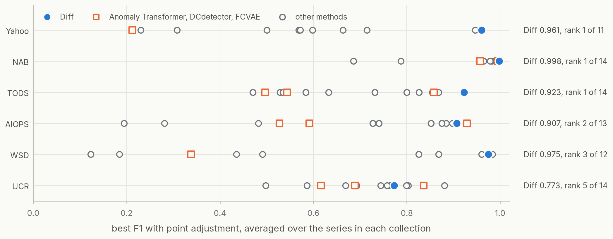
In this protocol each detector’s threshold is chosen per series to maximise F1 against the test labels, an optimistic choice applied to all detectors alike. The F1 is also computed after point adjustment: if any point inside a labelled anomalous segment is flagged, every point of that segment counts as detected [6].

Figure 2 looks at individual series, using plain pointwise F1 without point adjustment. On two Yahoo series, one threshold on Diff recovers the labels almost perfectly. On BIDMC1 from the UCR archive it fails badly. That series is a plethysmograph recording, the pulse wave of the blood, and its labelled anomaly is a premature ventricular contraction (an early heartbeat) that Wu and Keogh identified from an ECG recorded at the same time [1].

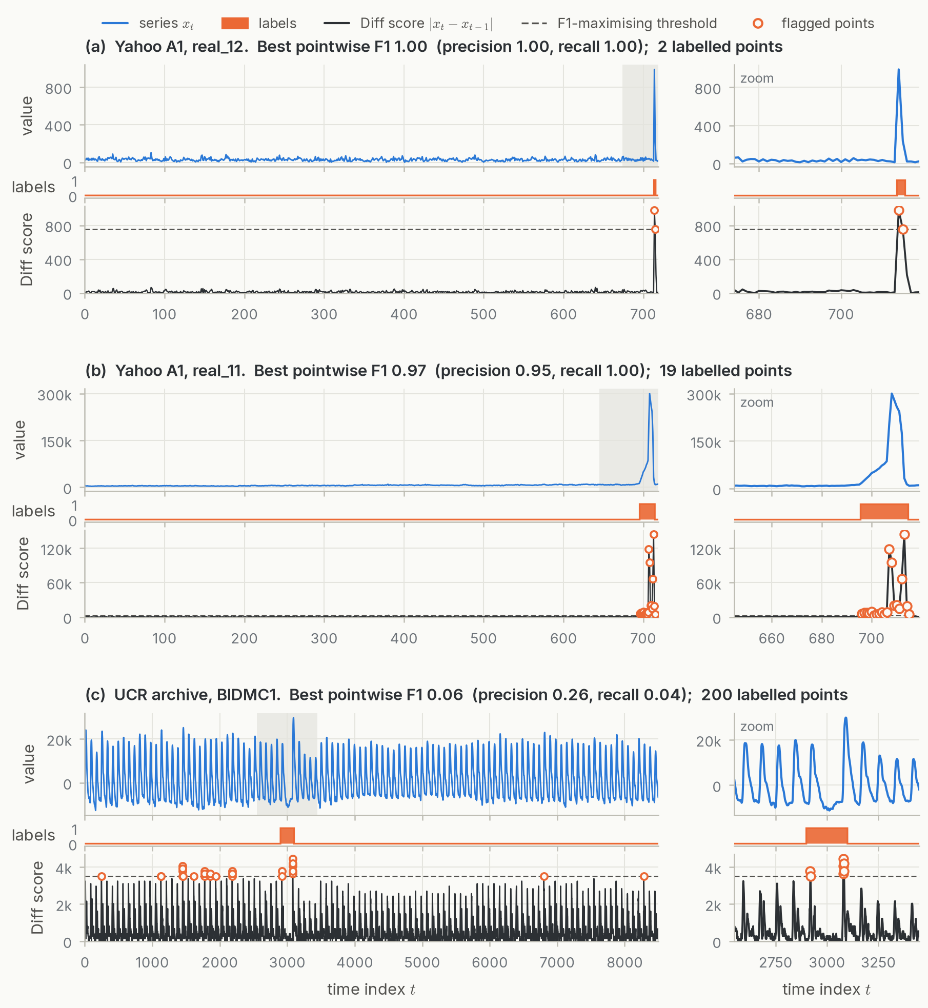
The derivation in Sections 2 to 4 accounts for the Yahoo series, and the information Diff discards, studied in Sections 5 and 6, accounts for the pulse recording. Sections 7 and 8 then use these results to examine evaluation, first the smallest error achievable from a given set of features and then the conditions under which a benchmark margin over Diff reflects a better detector.

02Notation

A series is $x_0,x_1,\dots$, one real number per time point. We write $\Delta x_t=x_t-x_{t-1}$ for the step into point $t$, and use the same notation for any sequence. EasyTSAD’s Diff score is $$s_0 = 0,\qquad s_t = |\Delta x_t| \quad (t\ge1).$$ It has no parameters, and a detector based on it flags $t$ when $s_t>\tau$.

Benchmarks label points, but Diff responds to steps, so our analysis labels steps: $Y_t=1$ means the step $\Delta x_t$ is anomalous. A single-point spike at $t$ then has two anomalous steps, into and out of $t$, while a jump to a new level has one. The two conventions differ for events that last many points, which Section 6 treats.

03When a Threshold on Diff Is Exact

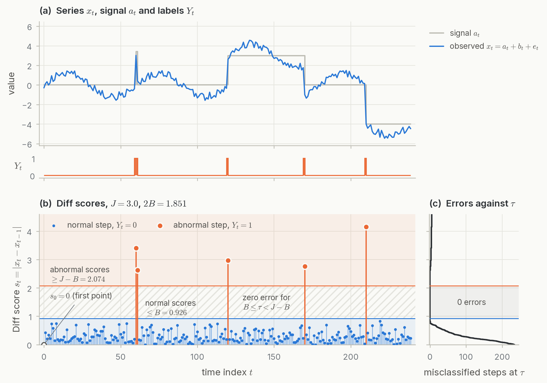
Write the series as $x_t=a_t+u_t$, where $a$ is the signal an annotator would call anomalous (a jump, a spike) and $u$ is what a healthy series does anyway, including trend, periodic structure and sensor noise. The split cannot be observed and serves only to describe the class of data on which Diff works. Assume that for every $t$ $$Y_t=0 \Rightarrow \Delta a_t = 0,\qquad Y_t=1 \Rightarrow |\Delta a_t| \ge J,\qquad |\Delta u_t| \le B.$$ On a normal step, $s_t=|\Delta u_t|\le B$. On an anomalous step, the nuisance can work against the jump but by at most $B$, so by the reverse triangle inequality $s_t=|\Delta a_t+\Delta u_t|\ge J-B$. Hence every threshold with $B\le\tau<J-B$ classifies every step correctly, and such a threshold exists if and only if $$J > 2B .$$ The argument uses no probability, so it also holds when the noise is dependent across time, as it usually is.

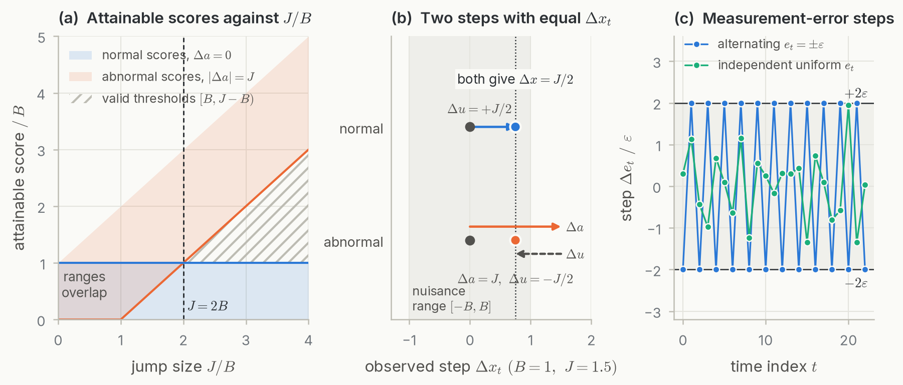
The constant $2$ cannot be improved, because if $J\le 2B$, a normal step with $\Delta u_t=J/2$ and an anomalous step with $\Delta a_t=J$, $\Delta u_t=-J/2$ both produce $\Delta x_t=J/2$, and no rule that sees only this step separates them (Figure 4b).

3.1What determines $B$

Split the nuisance further into a baseline $b$ with $|\Delta b_t|\le L$ and measurement error with $|e_t|\le\varepsilon$. Then $$|\Delta u_t| \le |\Delta b_t| + |e_t| + |e_{t-1}| \le L+2\varepsilon,$$ and the condition becomes $J>2L+4\varepsilon$. Differencing replaces a baseline by its per-step slope $L$, which is small for anything slow relative to the sampling rate, such as a daily cycle sampled every minute. It also counts the measurement error twice, and an error sequence alternating between $\pm\varepsilon$ attains the bound (Figure 4c). Figure 3 shows a constructed example.

04Random Noise

Sensor noise is rarely bounded, so we replace the bound $B$ by a tail condition. Fix a step and write $\Delta x_t=A+N$, with $A=0$ on normal steps, $|A|\ge J$ on anomalous ones, and $N$ the nuisance step. At the midpoint threshold $\tau=J/2$, a normal step is misclassified only if $|N|>J/2$, and an anomalous one only if $|A+N|\le J/2$, which again forces $|N|\ge J/2$. So every error lies in the event $\{|N|\ge J/2\}$, whatever the dependence between $A$, $Y$ and $N$.

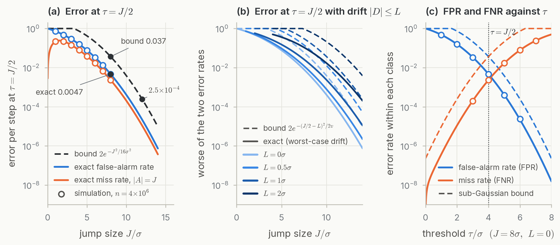
If $N$ is centred and sub-Gaussian with variance proxy $v$, meaning $\mathbb{E}\,e^{\lambda N}\le e^{v\lambda^2/2}$ for all $\lambda$, the Chernoff bound gives $$\Pr[\text{error}] \le \Pr\bigl[|N|\ge J/2\bigr] \le 2\exp\!\left(-\frac{J^2}{8v}\right).$$ For independent Gaussian sensor errors with standard deviation $\sigma$, $N=e_t-e_{t-1}$ has $v=2\sigma^2$ and the bound is $2e^{-J^2/16\sigma^2}$: about $2.5\times10^{-4}$ per step at $J=12\sigma$ and $0.037$ at $J=8\sigma$. At $J=8\sigma$ the exact Gaussian rates are about $0.005$ for false alarms and $0.002$ for misses. The miss rate is roughly half the false-alarm rate because only noise opposing the jump causes a miss, while a false alarm can come from either tail (Figure 5a).

A baseline step $D$ with $|D|\le L$ shifts the effective margin from $J/2$ to $J/2-L$, giving $2\exp(-(J/2-L)^2/2v)$ for $J\ge2L$ (Figure 5b).

Because anomalies are rare, we bound the two error rates separately. For $L\le\tau\le J-L$, $$\mathrm{FPR}(\tau) \le 2e^{-(\tau-L)^2/(2v)},\qquad \mathrm{FNR}(\tau) \le 2e^{-(J-\tau-L)^2/(2v)},$$ which makes the trade-off in $\tau$ explicit (Figure 5c). These bounds hold per step. Over a series of $T$ points the expected number of false alarms is $T\cdot\mathrm{FPR}$ by linearity, with no independence needed, so a $10^{-3}$ rate on a 10,000-point series still means about ten false alarms.

05Information Lost by Differencing

Computing Diff scores discards some information about a series, and no threshold or model trained on the scores can recover it.

Signed steps determine a series up to an additive constant: $\Delta x=\Delta z$ if and only if $z=x+c$. So nothing about the level of a series is available from its steps. A slow climb to a dangerous value produces only small steps. Whether such a climb is an anomaly is the labeller’s decision; Diff cannot distinguish it from a harmless drift.

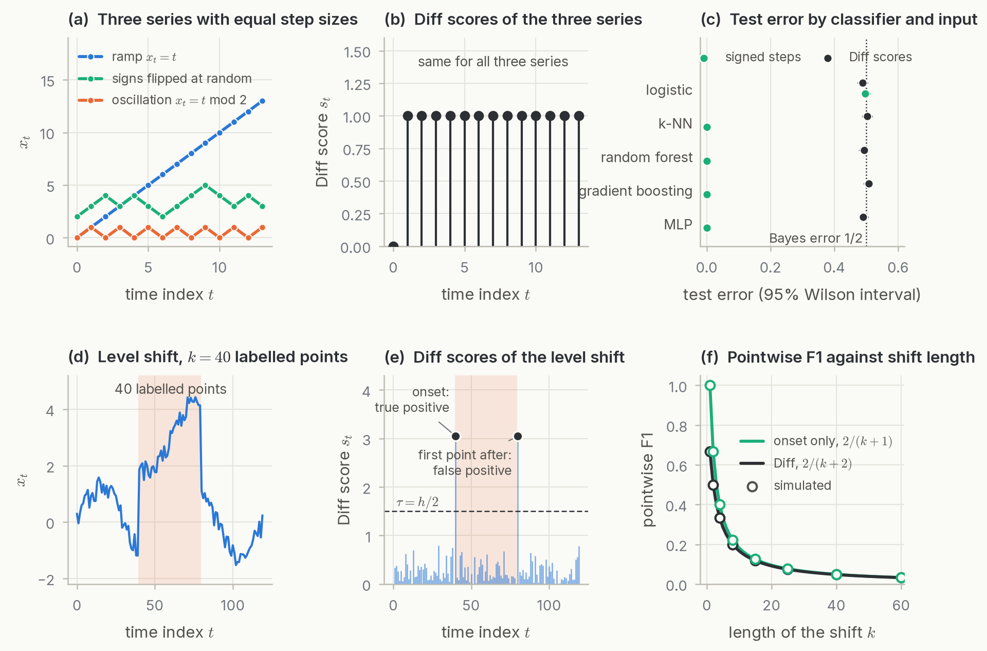
Taking absolute values also discards the sign of every step. Precisely, $s(x)=s(z)$ if and only if $\Delta z_t=\pm\Delta x_t$ at every $t$, with the sign chosen independently at each step. The ramp $0,1,2,3,\dots$ and the oscillation $0,1,0,1,\dots$ therefore have identical scores $0,1,1,1,\dots$. A task that labels the ramp normal and the oscillation anomalous, with equal prior probability, cannot be solved from the scores at better than error $1/2$. The same holds for any window of the two series, so a pointwise detector that looks at the scores in a neighbourhood of $t$ cannot do better either.

Figure 6c tests this with trained classifiers. One class of series moves monotonically (up or down with equal probability), the other alternates, and the step magnitudes are i.i.d. from the same distribution in both classes, so the score sequences are identically distributed across classes. On signed steps, k-NN, random forests, gradient boosting and an MLP reach zero test error, while on Diff scores all five classifiers stay at $1/2$. Logistic regression is at chance even on signed steps: any linear function of the steps takes values of both signs on the monotone class (whose sign is random) and values near zero on the alternating class, so no single cut on it separates them.

In general, a property of a series is a function of its Diff scores if and only if it is invariant under adding a constant and under flipping the sign of any subset of steps.

06Event Labels and the Pulse Recording

Diff fails on the pulse recording of Figure 2c for two reasons. Its precision is low because every normal heartbeat produces a pulse with a steep upstroke, so in the decomposition of Section 3 the regular beats belong to $u$, and $B$ is set by their steep edges. The pulse of the premature beat does produce the largest steps in the recording, but they exceed the normal pulses’ steps by far less than a factor of two. Any threshold low enough to catch more than its single largest step also catches normal pulses.

The 200-point annotation explains the low recall. It marks an abnormal state, while Diff responds to individual steps. Consider the cleanest version, a level shift of height $h$ held for $k$ points (Figure 6d,e). A threshold between the noise and $h$ flags the first point of the shift and the first point after it, giving $\mathrm{TP}=1$, $\mathrm{FP}=1$, $\mathrm{FN}=k-1$ and $$\mathrm{F1} = \frac{2}{k+2},$$ about $0.05$ for $k=40$, although the event was detected at its onset. A detector that flags only the onset gets $2/(k+1)$.

Point adjustment, used in Figure 1, was designed for this case: one flagged point inside a labelled segment credits the whole segment. It is why Diff averages $0.77$ on UCR there while scoring $0.06$ pointwise on BIDMC1. It also makes detection easy to overstate, since a detector that fires at random is likely to land inside every long segment; Kim et al. analyse this inflation and show that random scores can reach a high F1 under point adjustment [6].

07The Bayes Error of a Feature Map

The ramp and oscillation example is an instance of a general calculation that applies to any detector. Let $\phi$ be the features a detector sees (the Diff score at one point, the whole score sequence, or the raw series), and assume for simplicity that $\phi$ takes finitely many values. Inputs with the same value of $\phi$ must receive the same prediction, so the Bayes error of $\phi$ is $$\min_{g}\,\Pr\bigl[g(\phi(X))\ne Y\bigr] = \sum_{z}\min\bigl\{\Pr[\phi=z,\,Y=0],\;\Pr[\phi=z,\,Y=1]\bigr\},$$ attained by a majority vote within each level set of $\phi$. It is zero if and only if each value of $\phi$ occurs with one label only. For the ramp and oscillation, $\phi$ has a single value carrying probability $1/2$ under each label, so the Bayes error is $1/2$.

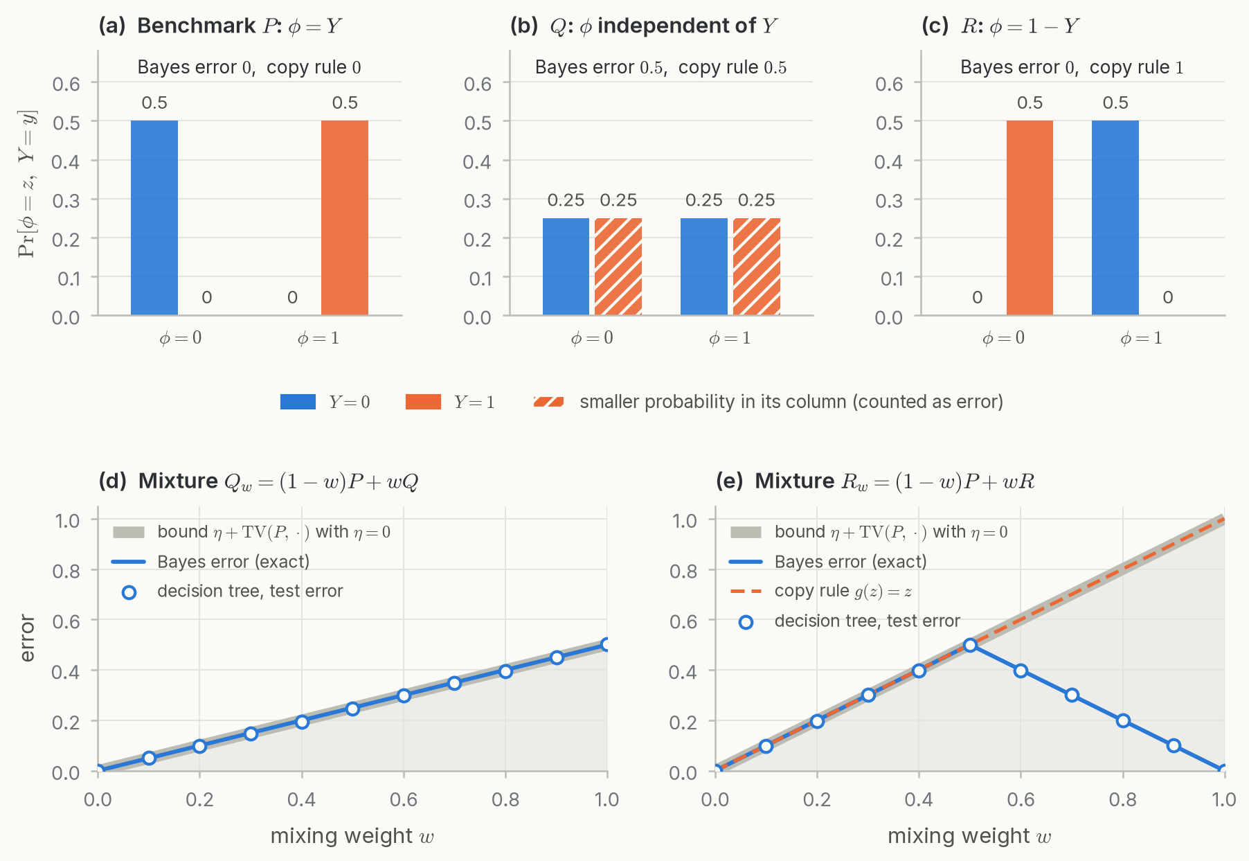
The masses in this sum belong to the joint distribution of features and labels, so the Bayes error depends on the dataset as well as on $\phi$. Diff’s near-perfect F1 on the Yahoo series of Figure 2 shows that the Bayes error of its score is small there and carries no information about data from another source, and an in-distribution test split cannot reveal the difference. Figure 7a–c shows a binary feature in three datasets. On the benchmark it equals the label (Bayes error $0$); on independent data its Bayes error is $1/2$; on data where the relation is reversed the Bayes error is $0$ again, yet the rule learned on the benchmark, $g(z)=z$, now errs everywhere, so the Bayes error and the error of the learned rule move in opposite directions.

To bound the change, let $P$ and $Q$ be the benchmark and deployment distributions over pairs $\omega=(\text{input},\text{label})$, let $\widetilde Y$ be the benchmark’s label and $Y$ the correct one, and let $\eta=\Pr_P[\widetilde Y\ne Y]$. With the total variation distance $\mathrm{TV}(P,Q)=\tfrac12\sum_\omega|P(\omega)-Q(\omega)|$, the Bayes error of $\phi$ under $(P,\widetilde Y)$ and under $(Q,Y)$ differ by at most $\eta+\mathrm{TV}(P,Q)$. Each relabelled point moves at most its own mass between the two minima in the sum, and changing the distribution moves at most $\mathrm{TV}$ of mass; this is the same mechanism as the classical domain-adaptation bounds [7]. Neither term is identifiable from the benchmark: $\eta$ requires correct labels and $\mathrm{TV}(P,Q)$ requires deployment data.

The bound is attained when the benchmark is mixed with the independent dataset: for $Q_w=(1-w)P+wQ$, $\mathrm{TV}(P,Q_w)=w/2$ and the Bayes error is exactly $w/2$ (Figure 7d). Mixing with the reversed dataset, $R_w=(1-w)P+wR$, gives Bayes error $\min(w,1-w)$, while the learned rule’s error grows linearly to $1$ (Figure 7e).

08Interpreting a Benchmark Margin

Suppose detector $a$ beats detector $b$ on a benchmark. We would like to conclude that $a$ has lower error on deployment data with correct labels. We use 0-1 error rather than F1 here because it decomposes over points, which makes the argument a few lines long; sampling error, label errors and distribution shift act on F1 in the same way, with the extra complication of a random denominator.

Only points where the two detectors disagree can affect the comparison. Where $a$ and $b$ output the same label they incur the same loss under any label and any distribution, so the per-point loss difference $\ell(a,\omega)-\ell(b,\omega)$ is in $\{-1,0,1\}$ and is nonzero only when $a(\omega)\ne b(\omega)$; on such a point, flipping the label changes it by $2$. Define $$\kappa_{ab}=\Pr_P\bigl[a\ne b,\ \widetilde Y\ne Y\bigr],\qquad \delta_{ab}=\sum_\omega |Q(\omega)-P(\omega)|\,\mathbf{1}\{a(\omega)\ne b(\omega)\}.$$ Then the error difference on $(Q,Y)$ and the error difference on $(P,\widetilde Y)$ differ by at most $2\kappa_{ab}+\delta_{ab}$. The factor 2 is the label flip; $\delta_{ab}$ has no $\tfrac12$ because the loss difference ranges over an interval of length 2 rather than 1. Adding the sampling error $m_{ab}$ between the test-set difference and its expectation under $(P,\widetilde Y)$, a measured margin larger than $m_{ab}+2\kappa_{ab}+\delta_{ab}$ certifies the ranking on deployment data.

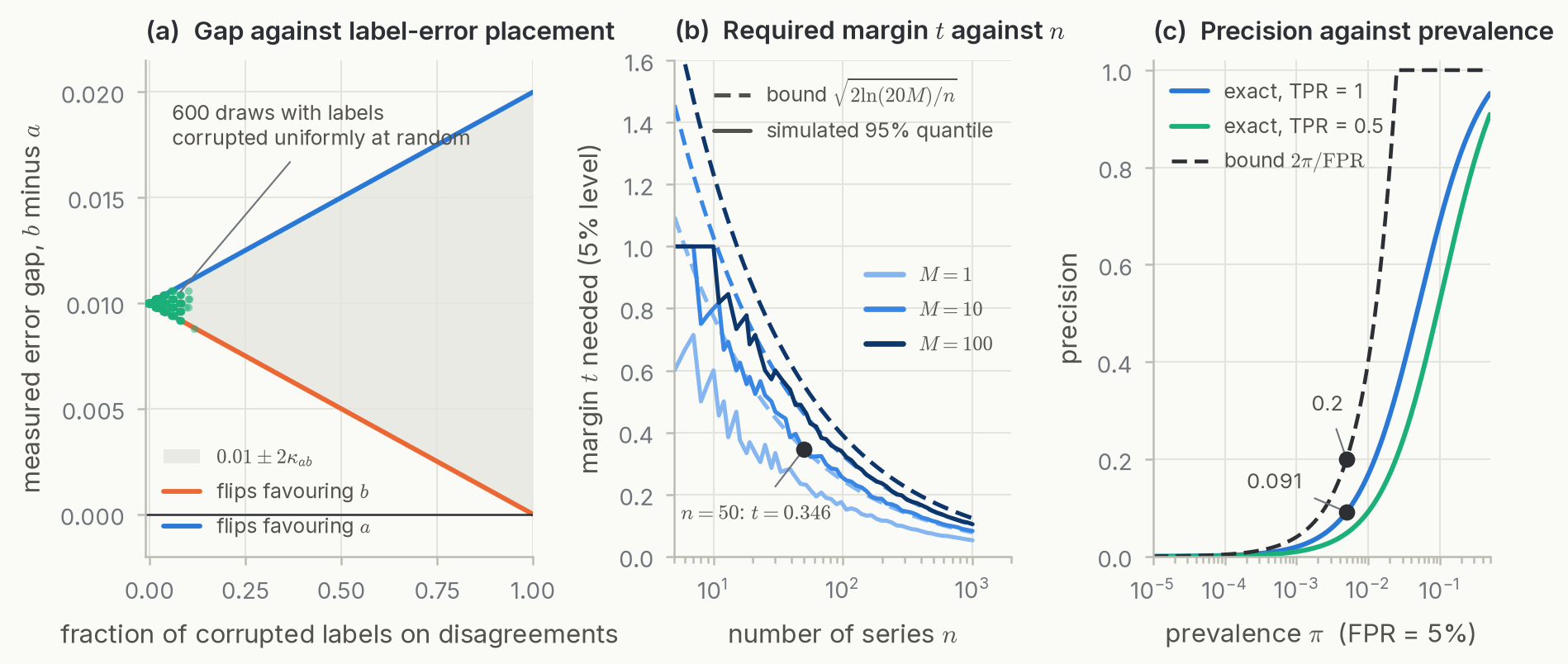
Both correction terms are supported on the disagreement set, which makes the bound usable in practice. Estimating $\kappa_{ab}$ only requires re-annotating the points where the two detectors disagree, typically a small fraction of the data. Suppose the detectors disagree on $3\%$ of points and $a$ leads by one percentage point. If $0.5\%$ of all labels are wrong and all of those fall on disagreements, $2\kappa_{ab}=0.01$ erases the lead; if they fall where the detectors agree, $\kappa_{ab}=0$. Label noise spread uniformly at random lands almost entirely on agreements and barely moves the comparison (Figure 8a).

For the sampling term, the independent unit is the series. Points within a series are strongly autocorrelated, and treating them as independent overstates the effective sample size. With $n$ series and per-series error differences in $[-1,1]$, Hoeffding’s inequality gives $m_{ab}\le t$ with probability at least $1-e^{-nt^2/2}$, so a one-sided 5% test needs $t=\sqrt{2\ln 20/n}$. That is $0.30$ for Yahoo A1’s 67 series and $0.15$ for the UCR archive’s 250. These are worst-case margins, since real per-series differences rarely use the full range, but a gap of a few F1 points is well below either. Selecting the best of $M$ thresholds or detectors on the same labels multiplies the failure probability by up to $M$ (union bound), giving $t=\sqrt{2\ln(20M)/n}$ (Figure 8b). The per-series oracle threshold in Figures 1 and 2 is such a selection, applied to every detector alike.

F1 itself is unstable when a series has few labelled points: one missing annotation can move a series from F1 1 to F1 0, and a detector that flags only the recorded anomalies outscores one that also finds unrecorded ones. Precision also depends on prevalence $\pi$: $$\text{precision} = \frac{\pi\,\mathrm{TPR}}{\pi\,\mathrm{TPR}+(1-\pi)\,\mathrm{FPR}} \le \frac{2\pi}{\mathrm{FPR}} \qquad (\pi\le\tfrac12).$$ At $\pi=0.5\%$ and $\mathrm{FPR}=5\%$, even perfect recall gives precision $50/548\approx0.091$ (in 10,000 points, 50 true alarms against about 498 false ones), and the bound caps it at $0.2$. Two detectors on the same collection share $\pi$, but averages across collections, and comparisons between papers that use different collections, mix very different prevalences (Figure 8c).

09Conclusions and Next Steps

Diff is exact whenever anomalies are steps more than twice the largest normal step, and under sub-Gaussian noise its error decays like $e^{-J^2/8v}$. The Yahoo series in Figure 2 have this form. We have not yet measured how much of each collection does, but Figure 1 suggests it is a large share for Yahoo, NAB and TODS under point-adjusted scoring. Diff fails when normal behaviour itself takes large steps, as in the pulse recording, and when labels mark long states, which point adjustment then partly hides.

For reading the literature, the consequence is that a margin of a few F1 points over Diff on these collections is weak evidence that a method detects anything Diff misses. Such a margin is within the sampling error of a few dozen series. Label errors on the small set of points where the two detectors disagree can produce or erase it, and switching between pointwise and adjusted scoring can change it.

Our next step is to test the assumptions above on real archives: measure step distributions at normal and anomalous points and test separation with thresholds fixed on held-out series, estimate the overlap of normal and anomalous score distributions (which bounds the Bayes error of Diff from below), re-annotate disagreement points between Diff and a stronger detector to estimate $\kappa_{ab}$, and repeat published comparisons with series as the sampling unit.

This is joint work with Vidyut Veedgav, Donovan Wu, Sreya Srinidhi and Weicong Chen. It grew out of our work on anomaly detection by estimating what typical data looks like, for images in Forte [8], for system logs in K⁴ [9] and its streaming deployment K4-Serve [10], and for language model prompts in Trust The Typical [11]. Diff’s results came up when we benchmarked that approach on time series.

References